2. Machine Learning

2.1. Supporting material

This chapter’s supporting material is Steve Brunton’s machine learning Primer:

Expanded explanation on types of machine learning tasks:

An introduction to neural networks—including a bit of the history of the model Neural Network Primer:

To develop a stronger intuition of how neural networks work: 3blue1brown Neural networks playlist:

2.2. Machine learning and Neuroscience

Machine learning —and specifically Deep Learning— holds great interest for neuroscientists, both as a research tool and as a set of algorithms that share similarities with the learning processes observed in biological brains. Machine learning models, particularly neural networks, are inspired by the structure and functionality of biological neural systems, making them an exciting area of study for understanding and potentially replicating aspects of brain function. These algorithms’ ability to learn complex patterns, adapt to new information, and generalize across different scenarios offers insights into the principles that may underlie human and animal learning. Additionally, machine learning can serve as a valuable tool for neuroscientists, enabling them to analyze large, complex datasets, model neural activity, and predict cognitive or behavioral outcomes. Thus, the intersection of machine learning and neuroscience not only facilitates the development of more advanced artificial intelligence systems but also contributes to our understanding of the brain and its remarkable learning capabilities.

Machine learning encompasses a variety of models and techniques that enable computers to learn from data and improve their performance over time. While neural networks have gained significant attention for their capabilities, there are numerous other models that cater to different problem types and requirements. Examples include linear regression, logistic regression, and support vector machines (SVMs) for continuous and categorical predictions, k-nearest neighbors (KNN) for instance-based learning, and clustering algorithms like k-means and DBSCAN for unsupervised learning tasks. Ensemble methods, such as random forests and gradient boosting machines, combine the outputs of multiple base models to improve prediction accuracy and stability. Additionally, Bayesian methods like Naïve Bayes and Gaussian processes facilitate probabilistic reasoning and uncertainty quantification. These diverse machine learning models, each with their own strengths and weaknesses, offer a rich toolkit for tackling a wide range of real-world problems, demonstrating that the field extends well beyond neural networks alone.

A machine learning task consist of three elements: the data, a model and an optimisation algorithm. Let’s first have a look at a few models:

2.3. Machine learning models

2.3.1. Decision trees

Decision trees are a popular and intuitive machine learning technique used for both classification and regression tasks. They function by recursively partitioning the data into subsets based on the feature values, ultimately forming a tree-like structure with decision nodes and leaf nodes. At each decision node, the algorithm selects the most informative feature to split the data, while the leaf nodes represent the final output or class labels. Decision trees offer a transparent and easily interpretable model, allowing users to visualize and understand the underlying decision-making process. However, they can be prone to overfitting, especially when the tree grows too deep. To mitigate this issue, techniques such as pruning can be employed to balance the model’s complexity and predictive power.

For many data applications, a type of decision tree model called boosted trees is often a better choice than neural networks. Boosted trees are an ensemble method that combines the predictions of multiple weak learners, usually shallow decision trees, to create a more robust and accurate model. Boosting algorithms, such as AdaBoost and Gradient Boosting, iteratively build these trees by focusing on the instances that are difficult to predict and assigning them higher importance in the subsequent tree construction. Boosted trees offer several advantages over neural networks, such as faster training times, easier interpretability, and lower susceptibility to overfitting. Furthermore, they generally perform well with smaller datasets and require less computational resources, making them a practical and powerful choice for a wide range of real-world data applications.

2.3.2. Deep learning

Deep learning is a subset of machine learning that focuses on multi-layered neural networks, known as “deep” neural networks, for representation learning. Although artificial neural networks trained with backpropagation first emerged in the 1980s, it wasn’t until 2012 that deep learning gained widespread attention. This occurred when a deep neural network trained on GPUs significantly outperformed non-deep learning methods in an annual image recognition competition. This accomplishment showcased that deep learning, in conjunction with fast hardware-accelerated implementations and large datasets, can yield exceptionally better results in non-trivial tasks compared to conventional methods. Consequently, researchers and practitioners rapidly adopted deep learning to tackle long-standing problems across various fields, including computer vision, natural language processing, reinforcement learning, and computational biology. This adoption led to numerous technological breakthroughs and state-of-the-art results in these domains.

2.3.2.1. MLP

Multilayer perceptrons (MLPs) are a class of feedforward artificial neural networks consisting of multiple layers of interconnected nodes or neurons. MLPs are organized into an input layer, one or more hidden layers, and an output layer. Each node within a layer is connected to every other node in the subsequent layer, forming a densely connected network. MLPs are capable of modeling complex, non-linear relationships within data, making them a versatile choice for various machine learning tasks, such as classification and regression. The learning process in MLPs involves adjusting the weights and biases of connections using an optimization algorithm like gradient descent in combination with backpropagation to compute the gradients. The incorporation of non-linear activation functions, such as the sigmoid or ReLU, allows MLPs to learn and represent non-linear mappings between inputs and outputs. Despite their simplicity compared to more advanced deep learning models, MLPs have proven to be effective in a wide range of applications and serve as a fundamental building block in the field of neural networks.

2.3.2.2. CNN

Convolutional neural networks (CNN), the deep neural network class, that is most commonly applied to image analysis and computer vision applications.

You’ve heard it before: images are made of pixels, so the CNN leverages the convolution operation to calculate latent (hidden) features for different pixels based on their surrounding pixel values. It does this by sliding a kernel (a.k.a. filter) over the input image and calculating the dot product between that small filter and the overlapping image area. This dot product leads to aggregate the neighboring pixel values to one representative scaler. Now let us twist our conceptualization of images a little bit and think of images as a graphs.

Convolutional neural networks are of special interest in neuroscience as there is extensive research studying the representational similarity between their activations and that of the human visual system.

Check out this interactive visualistion of the inner workings of a CNN caught in action classifying some digits.

2.3.3. Ensemble methods

Ensemble methods are a powerful approach in machine learning that leverage the collective wisdom of multiple base models to achieve more accurate and robust predictions. The underlying principle is that by combining diverse models, each with their own strengths and weaknesses, the ensemble can compensate for individual errors and capture a broader range of patterns in the data. This leads to improved overall performance and greater stability. Popular ensemble techniques include bagging, which averages the predictions of models trained on different random subsets of the data; boosting, which focuses on incrementally improving the performance of weak learners; and stacking, which uses a higher-level model to optimally combine the outputs of multiple base models. Ensemble methods have demonstrated success across a wide range of applications, offering a versatile and effective strategy for enhancing model performance in both classification and regression tasks.

2.3.4. Boosted decision trees vs deep learning

Choosing between boosted trees and neural networks depends on the problem, data characteristics, and desired outcomes. Boosted trees are often the preferred choice for structured data, such as tabular datasets, where the relationships between features are relatively simple. They offer advantages in terms of interpretability, computational efficiency, and resistance to overfitting, making them suitable for applications with limited data or resources. On the other hand, neural networks, particularly deep learning models, excel in handling complex, high-dimensional, and unstructured data, such as images, audio, or text. They are well-suited for tasks like image recognition, natural language processing, and speech recognition, where the ability to capture hierarchical representations is essential. Additionally, neural networks are more adept at modeling sequential or temporal dependencies, as seen in time-series analysis or text processing. Ultimately, the choice between boosted trees and neural networks should be guided by the specific problem, data, and requirements, weighing the trade-offs between performance, interpretability, and resource constraints.

2.4. Optimising the models

Optimization in the context of machine learning is the process of searching for the best values for the free parameters of a model, ensuring that it performs well on a given task. These free parameters, such as weights and biases in a neural network, determine the relationship between the input features and the output predictions. The goal of optimization is to minimize a predefined loss function, which quantifies the discrepancy between the model’s predictions and the actual target values. By iteratively updating the parameter values, the optimization algorithm navigates the model’s parameter space to find a set of values that yield the lowest possible loss. This process effectively tunes the model to capture underlying patterns and relationships in the data, ultimately improving its performance and generalization capabilities. The choice of optimization algorithm, along with appropriate hyperparameter settings, significantly impacts the efficiency and effectiveness of this search for optimal parameter values.

2.4.1. Gradient descent vs Backpropagation

Although often used interchangly in the context of deep learning, gradient descent and backpropagation are two distinct concepts.

Gradient descent is an optimization algorithm used for minimizing a loss function by iteratively updating the parameters of a model or a function. It operates by calculating the gradient of the loss function with respect to each parameter and adjusting the parameters in the direction of the negative gradient. The algorithm aims to find a set of parameter values that minimize the loss function.

On the other hand, backpropagation is a specific technique for computing the gradients of the loss function with respect to the parameters in a neural network. Backpropagation is the backbone optimization algorithm in modern machine learning, particularly for training deep neural networks. It is an efficient and elegant method for computing gradients of the loss function with respect to the model’s parameters, such as weights and biases. At its core, backpropagation involves the application of the chain rule from calculus to calculate partial derivatives, i.e. simple high-school mathematics. By iteratively adjusting the model’s parameters in the direction of the negative gradient, backpropagation minimizes the loss and improves the model’s performance. This simple yet powerful technique has been instrumental in the widespread adoption and success of neural networks across various domains, making it an essential component of contemporary machine learning.

2.5. Introduction to Machine learning with scikit-learn

Scikit-learn is a python library that allows to build many machine learning models with an simple interface. On the other hand, other ML libraries like Pytorch or Tensorflow are focused on machine with neural networks only.

We will use the same dataset we used on the previous notebook.

2.5.1. Data description

Each row represent a star.

Feature vectors:

• Temperature – The surface temperature of the star

• Luminosity – Relative luminosity: how bright it is

• Size – Relative radius: how big it is

• AM – Absolute magnitude: another measure of the star luminosity

• Color – General Color of Spectrum

• Type – Red Dwarf, Brown Dwarf, White Dwarf, Main Sequence , Super Giants, Hyper Giants

• Spectral_Class – O,B,A,F,G,K,M / SMASS - Stellar classification

import numpy as np
import matplotlib.pyplot as plt
import matplotlib
import pandas as pd
pd.options.mode.chained_assignment = None  

The DataFrame can be created from a csv file using the read_csv method. If you are working on Colab, you will need to upload the data.

df = pd.read_csv('Stars.csv')
df.head()

	Temperature	Luminosity	Size	A_M	Color	Spectral_Class	Type
0	3068	0.002400	0.1700	16.12	Red	M	Red Dwarf
1	3042	0.000500	0.1542	16.60	Red	M	Red Dwarf
2	2600	0.000300	0.1020	18.70	Red	M	Red Dwarf
3	2800	0.000200	0.1600	16.65	Red	M	Red Dwarf
4	1939	0.000138	0.1030	20.06	Red	M	Red Dwarf

from scipy import stats

r, p = stats.pearsonr(df['Temperature'], df['Temperature'])
print(f"The correlation coefficient is {r}")

The correlation coefficient is 0.9999999999999998

2.6. Supervised Learning

Supervised learning (SL) is the most common type of task in machine learning. It consist in finding a function that maps on space onto another, eg. the size of star to its luminosity. It can sub-divide into two types of task: regression and classification.

2.6.1. Regression

Let’s start by performing a regression (mapping one continual variable onto another one) on fake data so we make sure our set-up allows us to train models properly. We will generate the values from a sine function and train a neural network on them. Read the code line by line and make sure you understand what’s going on.

from sklearn.neural_network import MLPRegressor

# Generate data
X = np.linspace(0,20,5000).reshape(-1,1)  # X : a set of equally space between 0 and 50
Y = np.sin(X)                              # Y : the sine function for the X values

# Define neural network model
model = MLPRegressor(max_iter=200, # Maximum number of steps we update our model
                    activation="tanh",   # activation function
                    early_stopping=True,  # Should the training stop if loss converges? 
                    hidden_layer_sizes=(100,100), # Hidden layers size
                    )

# Train model by calling the .fit() method
model.fit(X, Y.ravel()) 

# Print Score: a score of 1 is a perfect fit
print('Score on training: ', model.score(X, Y))

# Predict data values with model and plot along original data
plt.figure(figsize=(16,10));
plt.scatter(X,Y, label='Original data');
input_x = np.linspace(X.min(), X.max(), 10000).reshape(-1,1)
pred_y = model.predict(input_x)
plt.plot(input_x,pred_y, label='Model prediction', color='red');
plt.legend(fontsize=16);

Score on training:  0.9987600798134659

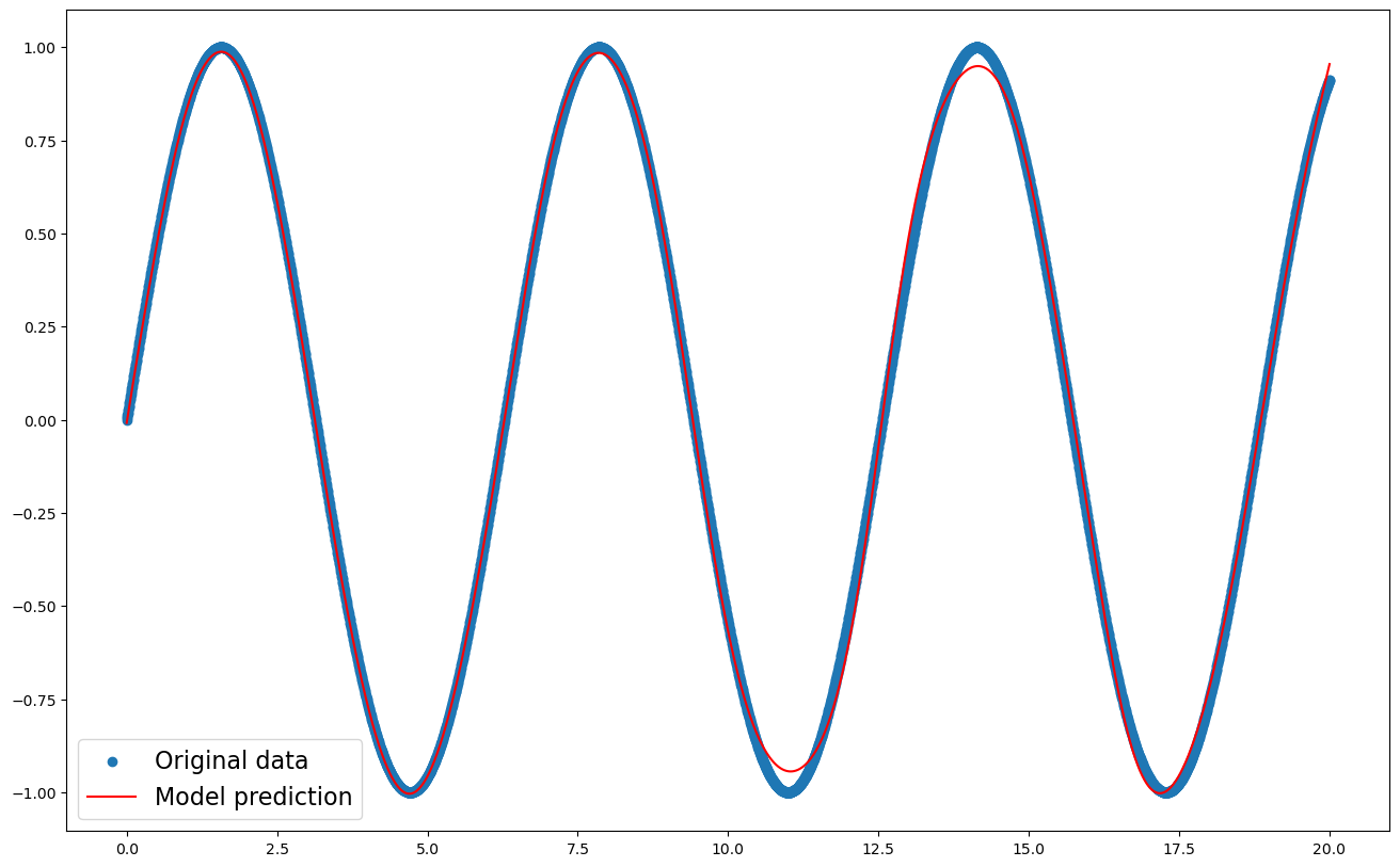
It seems to be working, the score should be close to 1.0 —which would be a perfect fit.

2.6.1.1. Exercise

• Extend the plot of the model we just trained so it predicts values outside of the range of those we used to train it. Does it still perform well on that range?

## Your code here

2.6.2. Real data

Moving on onto real data. Both the Luminosity and Absolute Magnitude relate to how bright a star is. Let’s try to figure out what the exact relation between them is. Let’s plot them.

df.plot.scatter('Luminosity','A_M', figsize=(16,10));

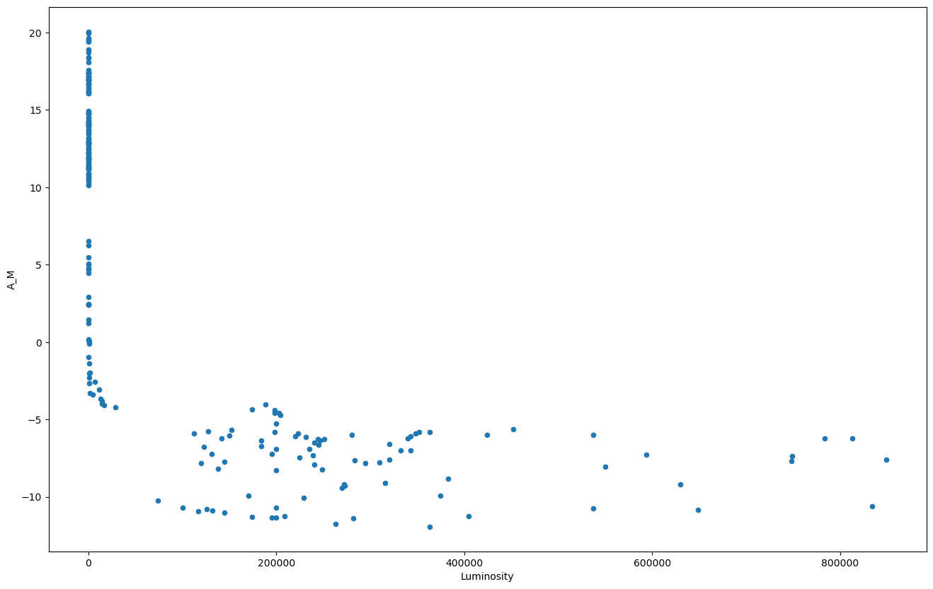
As you already knew, there is indeed a strong correlation between these two variables. You could even try to guess what the analytical formula is given the shape —or google it— but rather let’s see if we can instead build a model to predict the absolute magnitude for each luminosity. We could try a linear model but the relation is not quite linear, is it? Ie. it’s not a straight line. We could also try to fit a polynomial or a logarithmic function.. Instead we will build a neural network model so we don’t need to make any assumption about the relation between the variables.

We first need to import the library and models we are going to use:

from sklearn.neural_network import MLPRegressor
from sklearn.model_selection import train_test_split

We start by selecting the data and splitting it between training and test sets:

X = df['Luminosity'].values.reshape(-1,1) # Sklearn likes input data be given in a specific shape, don't worry too much about the reshape
Y = df['A_M'].values
X_train, X_test, y_train, y_test = train_test_split(X, Y, test_size=0.1)

We the initialise the model that we are going to train. We are gonna use a neural network, Sklearn deals with the details of making the neural network of the correct size for our data:

model = MLPRegressor(max_iter=1000, # Maximum number of steps we update our model
                    activation="tanh", # activation function
                    early_stopping=False, # Should the training stop if loss converges? 
                    hidden_layer_sizes=(300,300,300), # Hidden layers size
                    learning_rate_init=0.00005, # learning rate
                    learning_rate = 'adaptive',
                    )

Then, we simply need to call the method .fit() to train the model.

model.fit(X_train, y_train)

MLPRegressor(activation='tanh', hidden_layer_sizes=(300, 300, 300),
             learning_rate='adaptive', learning_rate_init=5e-05, max_iter=1000)

In a Jupyter environment, please rerun this cell to show the HTML representation or trust the notebook.
On GitHub, the HTML representation is unable to render, please try loading this page with nbviewer.org.

Let’s print the score:

print('Score on training set: ', model.score(X_train, y_train))
print('Score on test set: ', model.score(X_test, y_test))

Score on training set:  0.9107069502783415
Score on test set:  0.8566562516399513

Finally, let’s print our the data along with the values predicted by the model. We generate a set of luminosity values input_x and use the method model.prediction() to use our trained model to predict values.

df.plot.scatter('Luminosity','A_M', figsize=(16,10), label='Data', color='black');
input_x = np.linspace(0, X.max(), 100000).reshape(-1,1)
pred_y = model.predict(input_x)
plt.plot(input_x,pred_y, label='Model prediction', color='red');
plt.show();

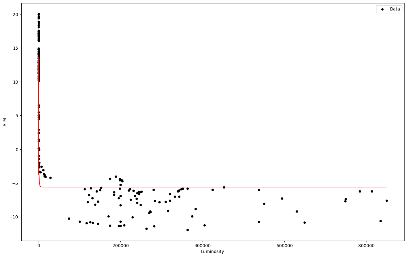
Congratulations, you just trained your first neural network on real data! The red line should hopefully fit the dataset points.

2.6.2.1. Exercise

• Train a neural network model to predict the absolute magnitude of the stars based on their temperature and size. Leave out 20% of the data as test set and evaluate the accuracy of the trained model on both the training set and the test set.

• Change the ratio of training vs test set. How does this affect the accuracy of the model?

## Your code here

2.6.3. Classification

Our dataset contains a categorical variable “Spectral Class”. This variable represents the color of the star. Let’s see if we could predict the spectral class of the stars based on the other features of the dataset.

Let’s visualise how many stars of each type there are in the data. If the amount of stars of one category was very small and another one too big, it would make the training quite difficult since the model would just learn to predict those over-represented in the data:

from matplotlib import cm
df.groupby('Type').size().plot(kind='pie', autopct='%.2f', cmap=cm.get_cmap('Spectral'), figsize=(16,16), fontsize=26);

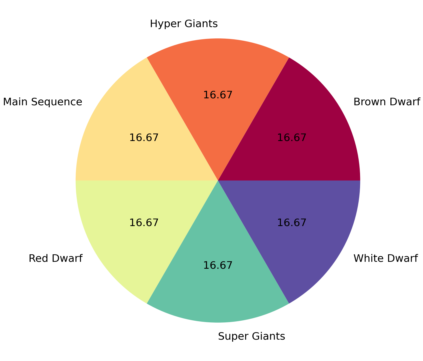
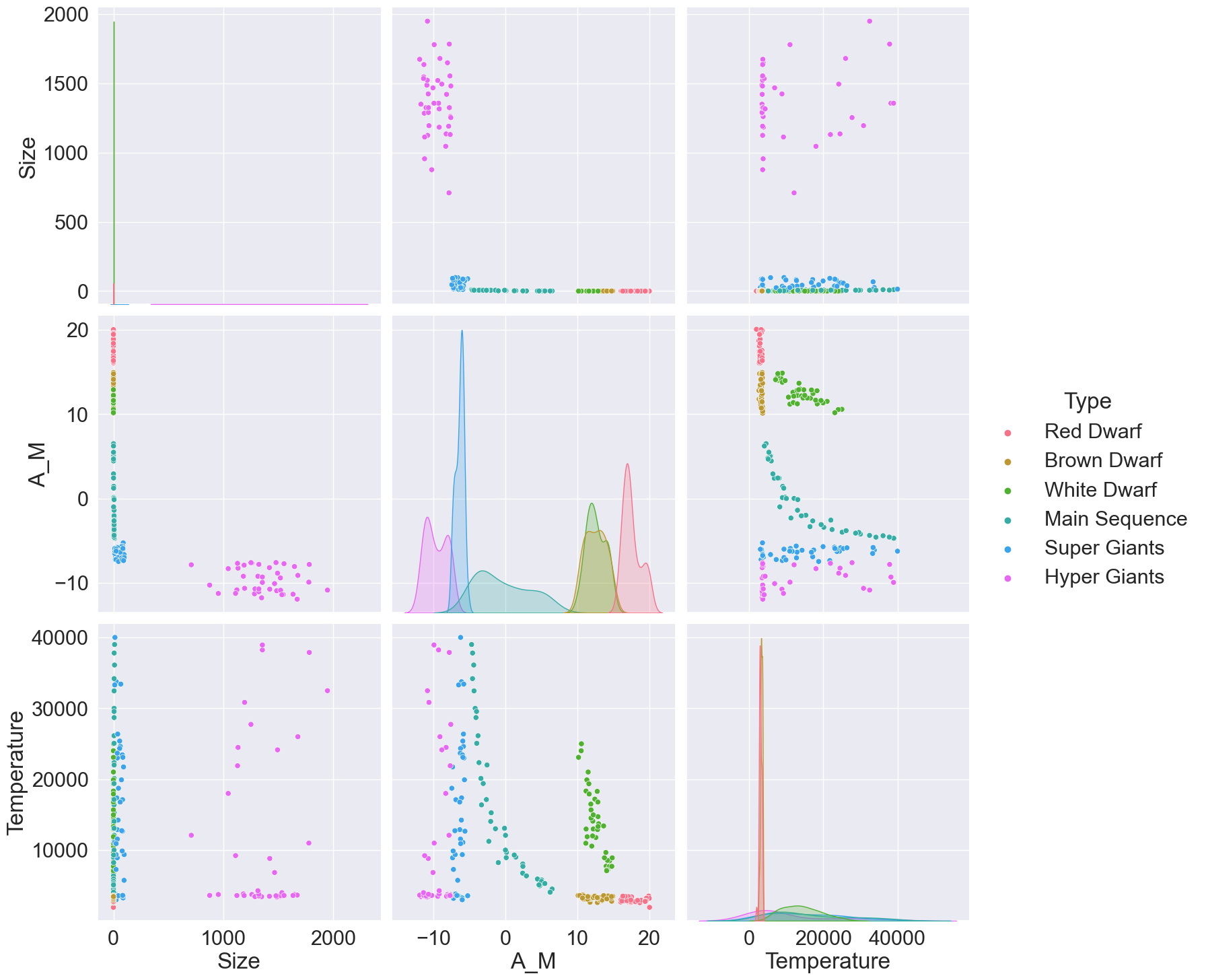
It seems the data is balanced with respect to stars types so we can safely move on. Let’s now visualise how the different variables relate to each other so we can pick features that would allow us to separate the stars based on their type:

import seaborn as sns# seaborn is a library similar to matplotlib but with some extra features and nicer default color schemes
sns.set(font_scale = 2)

features = ['Size', 'A_M', 'Temperature', 'Type']
sns.pairplot(df[features], hue="Type", palette="husl", height=5);

We start by selecting the data that we are gonna feed our model —the input— and the data that we want our model to predict —ie. to output—. In our case, we’re gonna try to predict the star type (White Dwarf, Super giants..) based on their temperature and absolute magnitude.

and the data that we want our model to predict —ie. to output—. In our case, we’re gonna try to predict the star type (White Dwarf, Super giants..) based on their temperature and absolute magnitude.

feature_cols = ['Temperature', 'A_M']
target_feature = 'Type'
X = df[feature_cols].values # 
Y = df[target_feature].values

We split the data between training data and test data:

random_seed = 9716 # This allow us to have reproducible results since both the splitting and training have stochastic component
X_train, X_test, y_train, y_test = train_test_split(X, Y, test_size=0.2, random_state=random_seed)

We can now train the model, we are going to use a neural network model MLPClassifier. So like usual, we import it and define its parameters:

from sklearn.neural_network import MLPClassifier

model = MLPClassifier(solver='adam', 
                    hidden_layer_sizes=(300,300,300), 
                    activation='tanh',
                    max_iter=10000,
                    learning_rate = 'adaptive',
                    learning_rate_init=0.00005,
                    early_stopping=False,
                    random_state = random_seed)

All that’s left is to train it by calling the .fit() method on the model. Beware, this might take some point to run.

model.fit(X_train, y_train)

print('Accuracy on training: ', model.score(X_train, y_train))
print('Accuracy on test: ', model.score(X_test, y_test))

Accuracy on training:  0.9322916666666666
Accuracy on test:  0.8541666666666666

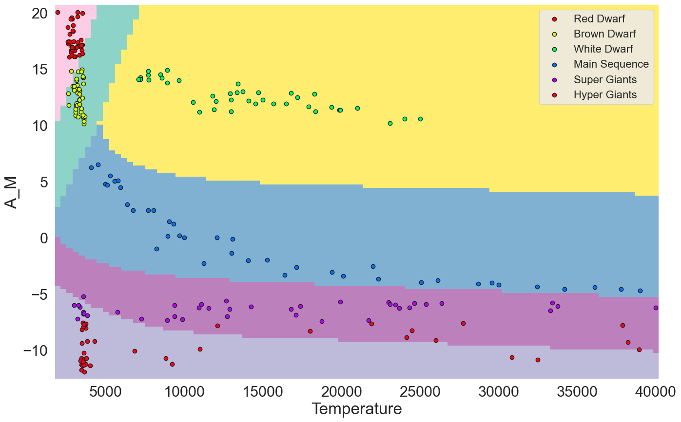
Since we are making predictions based on only two dimensions (temperature and absolute magnitude) we can make a figure with the decision boundaries for our model. To do so, we use Scikit-learn DecisionBoundaryDisplay function. ⚠️ It is possible that Google Colab doesn’t run the support the last version of Scipy which implements the DecisionBoundaryDisplay function. You will have to run this part locally on your computer or come talk to use to see what it looks like and just skip it.

from sklearn.inspection import DecisionBoundaryDisplay

DecisionBoundaryDisplay.from_estimator(
    model, # the model we just train
    X,     # the feature vectors we used to train the model
    cmap = 'Set3', 
    response_method="predict",
    plot_method="pcolormesh",
    shading="auto",
    xlabel=feature_cols[0],
    ylabel=feature_cols[1],
    eps=0.5,
);

# We plot the stars with each type on a different color
colors = plt.cm.get_cmap('hsv', len(df[target_feature].unique()))
for index, startype in enumerate(df[target_feature].unique()):
    stars_one_type = df[df[target_feature] == startype][feature_cols].values
    plt.scatter(stars_one_type[:, 0], stars_one_type[:, 1], color = colors(index), edgecolors="k", label=startype);

plt.legend(fontsize=16);
plt.show();

2.6.3.1. Exercise

• Use the predict() method of the model we just trained to predict the category of the stars with the following temperatures and absolute magnitude. Check that the predictions are compatible with those found in the Hertzsprung-Russell Diagram below. # Hint: you’ll need to add extra pair of brackets [[temperature value, absolute magnitude]] when calling the predict method of the model.

Temperature	Absolute Magnitude
7000	14
8000	4
4000	-7

## Your code here

• Train a neural network model to predict the Spectral Class of the stars, compute its accuracy and plot the decision boundaries (if you’re working locally). You can decide on which feature vectors you want to train the model as well as the size of your neural network model (argument hidden_layer_sizes in the model definition). # Hint: ML models models require manually tweaking the parameters, play with different network sizes until you get a good performance.

## Your code here

2.7. Bonus: Clustering

Cluster analysis or clustering consist in grouping objects such that the distance between similar objects is small while the distance between different objects is big. When objects are represented by high-dimensional data —think for instance of cell types represented by their proteomics or stars represented by their physical properties—, then the task of clustering becomes challenging.

Humans are great, but they have not evolved to easily understand and visualise high-dimensional data. To compensate this shortcoming, a first step when looking to cluster data is to reduce its dimensionality, meaning that we find some representation of the data in 2 or 3 dimension such that we obtain meaningful clusters.

The downside of performing dimensionality reduction is that there exist different low-dimensional representations of the same data. Therefore, finding which features of the data are relevant and how to project them to a low dimensional space is critical.

In the previous notebook, you have already done some manual clustering of some of the stars by simply selecting some range of the features —eg. temperature > 5000, certain luminosity, etc.— In this section we are gonna explore less manual approaches. Scikit-learn provides for a number of clustering algorithms, with K-Means being the go-to clustering method. K-Means computes clusters based on the similarity of the feature vectors.