Linear Algebra basics

Linear Algebra basics#

Credit: Ben Vanderlei’s Jupyter Guide to Linear Algebra and Damir Cavar notebooks under CC BY 4.0 with minor adaptations.

Supporting material#

This chapter’s supporting material is 3blue1brown Essence to Linear Algebra. You are encouraged to watch the whole playlist (it’s really good!) but specially relevant to this course are chapters 1 to 6 and chapters 14 to 16.

Concepts and Notation#

A scalar is an element in a vector, containing a real number value. In a vector space model or a vector mapping of (symbolic, qualitative, or quantitative) properties the scalar holds the concrete value or property of a variable.

A vector is an array, tuple, or ordered list of scalars (or elements) of size $n$ , with $n$ a positive integer. The length of the vector, that is the number of scalars in the vector, is also called the order of the vector.

A matrix is a list of vectors that all are of the same length. $A$ is a matrix with $m$ rows and $n$ columns, entries of $A$ are real numbers:

A \in R^{m \times n}

We use the notation $a_{i j}$ (or $A_{i j}$ , $A_{i, j}$ , etc.) to denote the entry of $A$ in the $i$ th row and $j$ th column:

\begin{array}{r} C = [\begin{array}{rrrr} a_{11} & a_{12} & \dots & a_{1 n} \\ a_{21} & a_{22} & \dots & a_{2 n} \\ ⋮ & ⋮ & ⋱ & ⋮ \\ a_{m 1} & a_{m 2} & \dots & a_{m n} \end{array}] \end{array}

A $n \times m$ matrix is a two-dimensional array with $n$ rows and $m$ columns.

A vector $x$ with $n$ entries of real numbers, could also be thought of as a matrix with $n$ rows and $1$ column, or as known as a column vector.

\begin{array}{r} x = [\begin{matrix} x_{1} \\ x_{2} \\ ⋮ \\ x_{n} \end{matrix}] \end{array}

Representing a row vector, that is a matrix with $1$ row and $n$ columns, we write $x^{T}$ (this denotes the transpose of $x$ , see above).

$x^{T} = [\begin{matrix} x_{1} & x_{2} & \dots & x_{n} \end{matrix}]$

Vector Spaces#

A vector space is a collection of objects, called vectors, together with definitions that allow for the addition of two vectors and the multiplication of a vector by a scalar. These operations produce other vectors in the collection and they satisfy a list of algebraic requirements such as associativity and commutativity. Although we will not consider the implications of each requirement here, we provide the list for reference.

For any vectors $U$ , $V$ , and $W$ , and scalars $p$ and $q$ , the definitions of vector addition and scalar multiplication for a vector space have the following properties:

$U + V = V + U$
$(U + V) + W = U + (V + W)$
$U + 0 = U$
$U + (- U) = 0$
$p (q U) = (p q) U$
$(p + q) U = p U + q U$
$p (U + V) = p U + p V$
$1 U = U$

The most familar example of vector spaces are the collections of single column arrays that we have been referring to as “vectors” throughout the previous chapter. The name given to the collection of all $n \times 1$ arrays is known as Euclidean $n$ -space, and is given the symbol $R^{n}$ . The required definitions of addition and scalar multiplication in $R^{n}$ are those described for matrices in Matrix Algebra. We will leave it to the reader to verify that these operations satisfy the list of requirements listed above.

The algebra of vectors by be visualized by interpreting the vectors as arrows. This is easiest to see with an example in $R^{2}$ .

\begin{array}{r} U_{1} = [\begin{matrix} 1 \\ 3 \end{matrix}] U_{2} = [\begin{matrix} 2 \\ - 1 \end{matrix}] \end{array}

The vector $U_{1}$ can be visualized as an arrow that points in the direction defined by 1 unit to the right, and 3 units up.

The algebra of vectors by be visualized by interpreting the vectors as arrows. This is easiest to see with an example in $R^{2}$ .

\begin{array}{r} U_{1} = [\begin{matrix} 1 \\ 3 \end{matrix}] U_{2} = [\begin{matrix} 2 \\ - 1 \end{matrix}] \end{array}

The vector $U_{1}$ can be visualized as an arrow that points in the direction defined by 1 unit to the right, and 3 units up.

%matplotlib inline
import numpy as np
import matplotlib.pyplot as plt

fig, ax = plt.subplots()
options = {"head_width":0.1, "head_length":0.2, "length_includes_head":True}

ax.arrow(0,0,1,3,fc='b',ec='b',**options)

ax.text(1,2,'$U_1$')

ax.set_xlim(0,5)
ax.set_ylim(0,5)
ax.set_aspect('equal')
ax.grid(True,ls=':')

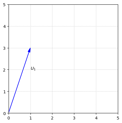
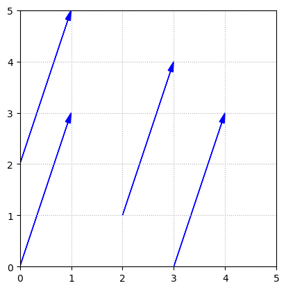
It is important to understand that it is the length and direction of this arrow that defines $U_{1}$ , not the actual position. We could draw the arrow in any number of locations, and it would still represent $U_{1}$ .

fig, ax = plt.subplots()

ax.arrow(0,0,1,3,fc='b',ec='b',**options)
ax.arrow(3,0,1,3,fc='b',ec='b',**options)
ax.arrow(0,2,1,3,fc='b',ec='b',**options)
ax.arrow(2,1,1,3,fc='b',ec='b',**options)

ax.set_xlim(0,5)
ax.set_ylim(0,5)
ax.set_aspect('equal')
ax.grid(True,ls=':')

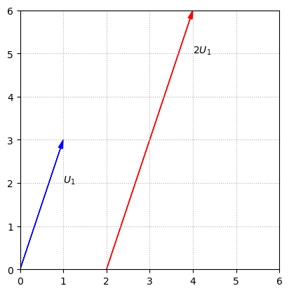
When we perform a scalar multiplication, such as $2 U_{1}$ , we interpret it as multiplying the length of the arrow by the scalar.

fig, ax = plt.subplots()

ax.arrow(0,0,1,3,fc='b',ec='b',**options)
ax.arrow(2,0,2,6,fc='r',ec='r',**options)

ax.text(1,2,'$U_1$')
ax.text(4,5,'$2U_1$')

ax.set_xlim(0,6)
ax.set_ylim(0,6)
ax.set_aspect('equal')
ax.grid(True,ls=':')

ax.set_xticks(np.arange(0,7,step = 1));
ax.set_yticks(np.arange(0,7,step = 1));

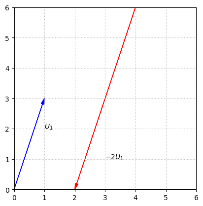
If the scalar is negative, we interpret the scalar multiplication as reversing the direction of the arrow, as well as changing the length.

fig, ax = plt.subplots()

ax.arrow(0,0,1,3,fc='b',ec='b',**options)
ax.arrow(4,6,-2,-6,fc='r',ec='r',**options)

ax.text(1,2,'$U_1$')
ax.text(3,1,'$-2U_1$')

ax.set_xlim(0,6)
ax.set_ylim(0,6)
ax.set_aspect('equal')
ax.grid(True,ls=':')

ax.set_xticks(np.arange(0,7,step = 1));
ax.set_yticks(np.arange(0,7,step = 1));

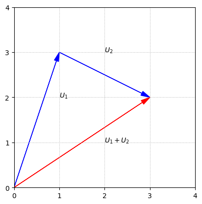
We can interpret the sum of two vectors as the result of aligning the two arrows tip to tail.

fig, ax = plt.subplots()

ax.arrow(0,0,1,3,fc='b',ec='b',**options)
ax.arrow(1,3,2,-1,fc='b',ec='b',**options)
ax.arrow(0,0,3,2,fc='r',ec='r',**options)

ax.text(1,2,'$U_1$')
ax.text(2,3,'$U_2$')
ax.text(2,1,'$U_1+U_2$')

ax.set_xlim(0,4)
ax.set_ylim(0,4)
ax.set_aspect('equal')
ax.grid(True,ls=':')

ax.set_xticks(np.arange(0,5,step = 1));
ax.set_yticks(np.arange(0,5,step = 1));

\begin{array}{r} [\begin{matrix} 1 \\ 3 \end{matrix}] + [\begin{matrix} 2 \\ - 1 \end{matrix}] = [\begin{matrix} 3 \\ 2 \end{matrix}] \end{array}

There are many other examples of vector spaces, but we will wait to provide these until after we have discussed more of the fundamental vector space concepts using $R^{n}$ as the setting.

Linear Systems#

In this first chapter, we examine linear systems of equations and seek a method for their solution. We also introduce the machinery of matrix algebra which will be necessary in later chapters, and close with some applications.

A linear system of $m$ equations with $n$ unknowns $x_{1}$ , $x_{2}$ , $x_{3}$ , … $x_{n}$ , is a collection of equations that can be written in the following form.

\begin{array}{r} \begin{array}{rcl} a_{11} x_{1} + a_{12} x_{2} + . . . + a_{1 n} x_{n} & = & b_{1} \\ a_{21} x_{1} + a_{22} x_{2} + . . . + a_{2 n} x_{n} & = & b_{2} \\ ⋮ ⋮ ⋮ & = & ⋮ \\ a_{m 1} x_{1} + a_{m 2} x_{2} + . . . + a_{m n} x_{n} & = & b_{m} \end{array} \end{array}

Solutions to the linear system are collections of values for the unknowns that satisfy all all of the equations simultaneously. The set of all possible solutions for the system is known as its solution set.

Linear systems with two equations and two unknowns are a great starting point since we easily graph the sets of points that satisfy each equation in the $x_{1} x_{2}$ coordinate plane. The set of points that satisfy a single linear equation in two variables forms a line in the plane. Three examples will be sufficient to show the possible solution sets for linear systems in this setting.

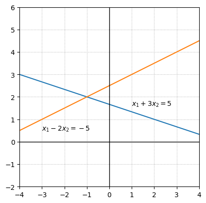
Example 1: System with a unique solution#

\begin{array}{r} \begin{array}{rcl} x_{1} + 3 x_{2} & = & 5 \\ x_{1} - 2 x_{2} & = & - 5 \end{array} \end{array}

The solution set for each equation can be represented by a line, and the solution set for the linear system is represented by all points that lie on both lines. In this case the lines intersect at a single point and there is only one pair of values that satisfy both equations, $x_{1} = - 1$ , $x_{2} = 2$ .

%matplotlib inline
import numpy as np
import matplotlib.pyplot as plt

x=np.linspace(-5,5,100)

fig, ax = plt.subplots()
ax.plot(x,(5-x)/3)
ax.plot(x,(5+x)/2)

ax.text(1,1.6,'$x_1+3x_2 = 5$')
ax.text(-3,0.5,'$x_1-2x_2 = -5$')

ax.set_xlim(-4,4)
ax.set_ylim(-2,6)
ax.axvline(color='k',linewidth = 1)
ax.axhline(color='k',linewidth = 1)

## This options specifies the ticks based the list of numbers provided.
ax.set_xticks(list(range(-4,5)))
ax.set_aspect('equal')
ax.grid(True,ls=':')

We are looking for a unique solution for the two variables $x_{1}$ and $x_{2}$ . The system can be described as $A x = b$ with the matrices :

\begin{array}{r} A = [\begin{array}{rr} 1 & 3 \\ 1 & - 2 \end{array}], b = [\begin{array}{rr} 5 \\ - 5 \end{array}] \end{array}

Exercises#

-Are the solution to the above system of equations scalars or vectors?

## Dicuss the question with your group mates. Ask us in case of doubts :)

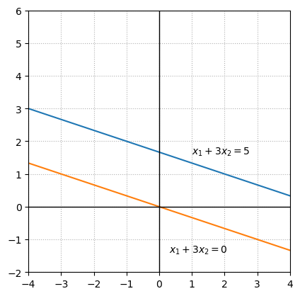
Example 2: System with no solutions#

\begin{array}{r} \begin{array}{rcl} x_{1} + 3 x_{2} & = & 5 \\ x_{1} + 3 x_{2} & = & 0 \end{array} \end{array}

In this example the solution sets of the individual equations represent lines that are parallel. There is no pair of values that satisfy both equations simultaneously.

fig, ax = plt.subplots()
ax.plot(x,(5-x)/3)
ax.plot(x,-x/3)

ax.text(1,1.6,'$x_1+3x_2 = 5$')
ax.text(0.3,-1.4,'$x_1+3x_2 = 0$')

ax.set_xlim(-4,4)
ax.set_ylim(-2,6)
ax.axvline(color='k',linewidth = 1)
ax.axhline(color='k',linewidth = 1)

## This options specifies the ticks based the list of numbers provided.
ax.set_xticks(list(range(-4,5)))
ax.set_aspect('equal')
ax.grid(True,ls=':')

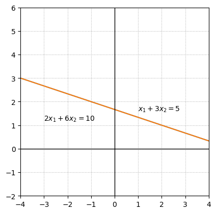
Example 3: System with an infinite number of solutions#

\begin{array}{r} \begin{array}{rcl} x_{1} + 3 x_{2} & = & 5 \\ 2 x_{1} + 6 x_{2} & = & 10 \end{array} \end{array}

In the final example, the second equation is a multiple of the first equation. The solution set for both equations is represented by the same line and thus every point on the line is a solution to the linear system.

fig, ax = plt.subplots()
ax.plot(x,(5-x)/3)
ax.plot(x,(5-x)/3)

ax.text(1,1.6,'$x_1+3x_2 = 5$')
ax.text(-3,1.2,'$2x_1+6x_2 = 10$')

ax.set_xlim(-4,4)
ax.set_ylim(-2,6)
ax.axvline(color='k',linewidth = 1)
ax.axhline(color='k',linewidth = 1)

ax.set_xticks(list(range(-4,5)))
ax.set_aspect('equal')
ax.grid(True,ls=':')

These examples illustrate all of the possibile types of solution sets that might arise in a system of two equations with two unknowns. Either there will be exactly one solution, no solutions, or an infinite collection of solutions. A fundamental fact about linear systems is that their solution sets are always one of these three cases.

Inverse Matrices#

In this section we consider the idea of inverse matrices and describe a common method for their construction.

As a motivation for the idea, let’s again consider the system of linear equations written in the matrix form.

A X = B

Again, $A$ is a matrix of coefficients that are known, $B$ is a vector of known data, and $X$ is a vector that is unknown. If $A$ , $B$ , and $X$ were instead only numbers, we would recognize immediately that the way to solve for $X$ is to divide both sides of the equation by $A$ , so long as $A \neq 0$ . The natural question to ask about the system is Can we define matrix division?

The answer is Not quite. We can make progress though by understanding that in the case that $A$ , $B$ , and $X$ are numbers, we could also find the solution by multiplying by $1 / A$ . This subtle distinction is important because it means that we do not need to define division. We only need to find the number, that when multiplied by $A$ gives 1. This number is called the multiplicative inverse of $A$ and is written as $1 / A$ , so long as $A \neq 0$ .

We can extend this idea to the situation where $A$ , $B$ , and $X$ are matrices. In order to solve the system $A X = B$ , we want to multiply by a certain matrix, that when multiplied by $A$ will give the identity matrix $I$ . This matrix is known as the inverse matrix, and is given the symbol $A^{- 1}$ .

If $A$ is a square matrix we define $A^{- 1}$ (read as “A inverse”) to be the matrix such that the following are true.

A^{- 1} A = I A A^{- 1} = I

Notes about inverse matrices:

The matrix must be square in order for this definition to make sense. If $A$ is not square, it is impossible for both $A^{- 1} A$ and $A A^{- 1}$ to be defined.
Not all matrices have inverses. Matrices that do have inverses are called invertible matrices. Matrices that do not have inverses are called non-invertible, or singular, matrices.
If a matrix is invertible, its inverse is unique.

Now if we know $A^{- 1}$ , we can solve the system $A X = B$ by multiplying both sides by $A^{- 1}$ .

A^{- 1} A X = A^{- 1} B

Then $A^{- 1} A X = I X = X$ , so the solution to the system is $X = A^{- 1} B$ . Unfortunately, it is typically not easy to find $A^{- 1}$ .

Construction of an inverse matrix#

We take $C$ as an example matrix, and consider how we might build the inverse.

\begin{array}{r} C = [\begin{array}{rrrr} 1 & 0 & 2 & - 1 \\ 3 & 1 & - 3 & 2 \\ 2 & 0 & 4 & 4 \\ 2 & 1 & - 1 & - 1 \end{array}] \end{array}

Let’s think of the matrix product $C C^{- 1} = I$ in terms of the columns of $C^{- 1}$ . We put focus on the third column as an example, and label those unknown entries with $y_{i}$ . The * entries are uknown as well, but we will ignore them for the moment.

\begin{array}{r} C C^{- 1} = [\begin{array}{rrrr} 1 & 0 & 2 & - 1 \\ 3 & 1 & - 3 & 2 \\ 2 & 0 & 4 & 4 \\ 2 & 1 & - 1 & - 1 \end{array}] [\begin{array}{rrrr} * & * & y_{1} & * \\ * & * & y_{2} & * \\ * & * & y_{3} & * \\ * & * & y_{4} & * \end{array}] = [\begin{array}{rrrr} 1 & 0 & 0 & 0 \\ 0 & 1 & 0 & 0 \\ 0 & 0 & 1 & 0 \\ 0 & 0 & 0 & 1 \end{array}] = I \end{array}

Recall now that $C$ multiplied by the third column of $C^{- 1}$ produces the third column of $I$ . This gives us a linear system to solve for the $y_{i}$ .

\begin{array}{r} [\begin{array}{rrrr} 1 & 0 & 2 & - 1 \\ 3 & 1 & - 3 & 2 \\ 2 & 0 & 4 & 4 \\ 2 & 1 & - 1 & - 1 \end{array}] [\begin{matrix} y_{1} \\ y_{2} \\ y_{3} \\ y_{4} \end{matrix}] = [\begin{matrix} 0 \\ 0 \\ 1 \\ 0 \end{matrix}] \end{array}

Exercises#

Write down the matrix $C$ using a numpy array

## Code solution here
# C = ...

Inverse matrices with SciPy#

The $inv$ function is used to compute inverse matrices in the SciPy $linalg$ module. Once the module is imported, the usage of $inv$ is exactly the same as the function we just created.

from scipy import linalg

C_inverse = linalg.inv(C)
print(C_inverse)

## Your solution here

---------------------------------------------------------------------------
NameError                                 Traceback (most recent call last)
Cell In[12], line 3
      1 from scipy import linalg
----> 3 C_inverse = linalg.inv(C)
      4 print(C_inverse)

NameError: name 'C' is not defined

Verify that C_inverse is indeed the inverse matrix of C by verifying that C@C_inverse is the identity matrix

## Your solution here

Providing a non-invertible matrix to $inv$ will result in an error being raised by the Python interpreter.

Exercises#

Let $A$ and $B$ be two random $4 \times 4$ matrices. Demonstrate using Python that $(A B)^{- 1} = B^{- 1} A^{- 1}$ for the matrices.

## Code solution here

Discuss with your group mates what is the geometrical meaning of a matrix that can be inverted and a matrix that can not be inverted. Hint: remeber from the 3Blue1Brown videos that a matrix can represent a linear transformation.

Linear Combinations#

At the core of many ideas in linear algebra is the concept of a linear combination of vectors. To build a linear combination from a set of vectors ${V_{1}, V_{2}, V_{3}, . . . V_{n}}$ we use the two algebraic operations of addition and scalar multiplication. If we use the symbols $a_{1}, a_{2}, . . ., a_{n}$ to represent the scalars, the linear combination looks like the following.

a_{1} V_{1} + a_{2} V_{2} + a_{3} V_{3} + . . . . + a_{n} V_{n}

The scalars $a_{1}, a_{2}, . . ., a_{n}$ are sometimes called weights.

Let’s define a collection of vectors to give concrete examples.

\begin{array}{r} V_{1} = [\begin{matrix} 2 \\ - 2 \\ 1 \end{matrix}] V_{2} = [\begin{matrix} 1 \\ 0 \\ - 1 \end{matrix}] V_{3} = [\begin{matrix} 0 \\ - 1 \\ 6 \end{matrix}] \end{array}

Now $3 V_{1} + 2 V_{2} + 4 V_{3}$ , $V_{1} - V_{2} + V_{3}$ , and $3 V_{2} - V_{3}$ are all examples of linear combinations of the set of vectors ${V_{1}, V_{2}, V_{3}}$ and can be calculated explicitly if needed.

\begin{array}{r} 3 V_{1} + 2 V_{2} + 4 V_{3} = 3 [\begin{matrix} 2 \\ - 2 \\ 1 \end{matrix}] + 2 [\begin{matrix} 1 \\ 0 \\ - 1 \end{matrix}] + 4 [\begin{matrix} 0 \\ - 1 \\ 6 \end{matrix}] = [\begin{matrix} 8 \\ - 10 \\ 25 \end{matrix}] \end{array}

The concept of linear combinations of vectors can be used to reinterpret the problem of solving linear systems of equations. Let’s consider the following system.

\begin{array}{r} \begin{array}{rcl} x_{1} + 2 x_{2} & = & 0 \\ 3 x_{1} - x_{2} & = & 14 \end{array} \end{array}

We’ve already discussed how this system can be written using matrix multiplication.

\begin{array}{r} [\begin{array}{cc} 1 & 2 \\ 3 & - 1 \end{array}] [\begin{array}{c} x_{1} \\ x_{2} \end{array}] = [\begin{array}{c} 0 \\ 14 \end{array}] \end{array}

We’ve also seen how this matrix equation could be repackaged as a vector equation.

\begin{array}{r} x_{1} [\begin{matrix} 1 \\ 3 \end{matrix}] + x_{2} [\begin{matrix} 2 \\ - 1 \end{matrix}] = [\begin{matrix} 0 \\ 14 \end{matrix}] \end{array}

The connection to linear combinations now becomes clear if we consider the columns of the coefficient matrix as vectors. Finding the solution to the linear system of equations is equivalent to finding the linear combination of these column vectors that matches the vector on the right hand side of the equation.

Exercises#

Use scipy function linalg.solve() to solve the above sytem, that is, to find the values $x_{1}$ and $x_{2}$ that makes the above equation true. Hint: You can check how to use scipy function in the scipy documentation.

## Your solution here

Use python to check that the obtained solution values for $x_{1}$ and $x_{2}$ is verified by performing the operation

$x_{1} [\begin{array}{r} 1 \\ 3 \end{array}] + x_{2} [\begin{array}{r} 2 \\ - 1 \end{array}]$ and checking that the result is $[\begin{array}{r} 0 \\ 14 \end{array}]$

## Your solution here

Linear Independence#

A set of vectors ${V_{1}, V_{2}, V_{3}, . . . V_{n}}$ is said to be linearly independent if no linear combination of the vectors is equal to zero, except the combination with all weights equal to zero. Thus if the set is linearly independent and

c_{1} V_{1} + c_{2} V_{2} + c_{3} V_{3} + . . . . + c_{n} V_{n} = 0

it must be that $c_{1} = c_{2} = c_{3} = . . . . = c_{n} = 0$ . Equivalently we could say that the set of vectors is linearly independent if there is no vector in the set that is equal to a linear combination of the others. If a set of vectors is not linearly independent, then we say that it is linearly dependent.

Example 1: Vectors in $R^{2}$ #

\begin{array}{r} V_{1} = [\begin{matrix} 2 \\ 1 \end{matrix}] V_{2} = [\begin{matrix} 1 \\ - 6 \end{matrix}] \end{array}

In order to determine if this set of vectors is linearly independent, we must examine the following vector equation.

\begin{array}{r} c_{1} [\begin{matrix} 2 \\ 1 \end{matrix}] + c_{2} [\begin{matrix} 1 \\ - 6 \end{matrix}] = [\begin{matrix} 0 \\ 0 \end{matrix}] \end{array}

Exercises#

Use scipy function linalg.solve() to solve the above sytem, that is, to find the values $c_{1}$ and $c_{2}$ that makes the above equation true. Hint: You can check how to use scipy function in the scipy documentation.

## Hint: think of the geometrical interpretation of the system of two equations as two straight lines.

## Your solution here

Homogeneous systems#

A linear system is said to be homogeneous if it can be described with the matrix equation $A X = 0$ . The solution to such a system has a connection to the solution of the system $A X = B$ . The homogeneous system also has a connection to the concept of linear independence. If we link all of these ideas together we will be able to gain information about the solution of the system $A X = B$ , based on some information about linear independence.

In the previous examples we were solving the vector equation $c_{1} V_{1} + c_{2} V_{2} + c_{3} V_{3} + . . . . + c_{n} V_{n} = 0$ in order to determine if the set of vectors ${V_{1}, V_{2}, V_{3} . . . . V_{n}}$ were linearly independent. This vector equation represents a homogeneous linear system that could also be described as $A X = 0$ , where $V_{1}$ , $V_{2}$ , … $V_{n}$ are the columns of the matrix $A$ , and $X$ is the vector of unknown coefficients. The set of vectors is linearly dependent if and only if the associated homogeneous system has a solution other than the vector with all entries equal to zero. The vector of all zeros is called the trivial solution. This zero vector is called a trivial solution because it is a solution to every homogeneous system $A X = 0$ , regardless of the entries of $A$ . For this reason, we are interested only in the existence of nontrivial solutions to $A X = 0$ .

Let us suppose that a homogeneous system $A X = 0$ has a nontrivial solution, which we could label $X_{h}$ . Let us also suppose that a related nonhomogeneous system $A X = B$ also has some particular solution, which we could label $X_{p}$ . So we have $A X_{h} = 0$ and $A X_{p} = B$ . Now by the properties of matrix multiplication, $X_{p} + X_{h}$ is also a solution to $A X = B$ since $A (X_{p} + X_{h}) = A X_{p} + A X_{h} = B + 0$ .

Consider the following system as an example.

\begin{array}{r} A X = [\begin{array}{rrr} - 3 & 2 & 1 \\ - 2 & 1 & - 1 \\ 4 & 3 & 3 \end{array}] [\begin{matrix} x_{1} \\ x_{2} \\ x_{3} \end{matrix}] = [\begin{matrix} - 6 \\ 1 \\ 13 \end{matrix}] = B \end{array}

We can look at the associated homogeneous system to determine if the columns of $A$ are linearly independent.

\begin{array}{r} [\begin{array}{rrr} - 3 & 2 & 1 \\ - 2 & 1 & - 1 \\ 4 & 3 & 3 \end{array}] [\begin{matrix} c_{1} \\ c_{2} \\ c_{3} \end{matrix}] = [\begin{matrix} 0 \\ 0 \\ 0 \end{matrix}] \end{array}

Rank and Number of solutions of a system#

The rank of a system of linear equations is the maximal number of linearly independent vectors. If the rank is smaller than the number of vectores, then some vectors are linearly dependent: ie. they can be written as a linear combination of two other vectors.

If $r a n k (A) = r a n k ([A | b])$ then the system Ax = b has a solution.
If $r a n k (A) = r a n k ([A | b]) = n$ then the system Ax = b has a unique solution.
If $r a n k (A) = r a n k ([A | b]) < n$ then the system Ax = b has infinitely many solutions.
If $r a n k (A) < r a n k ([A | b])$ then the system Ax = b is inconsistent; i.e., b is not in C(A).

Exercises#

Use the same scipy function as above to solve the homogenous and the non-homogenous systems above. Do they have the same set of solutions? Did you expect that?

## Code solution here.

Null space#

With the concept of homogeneous systems in place, we are ready to define the second fundamental subspace. If $A$ is an $m \times n$ matrix, the null space or nullity of $A$ is the set of vectors $X$ , such that $A X = 0$ . In other words, the null space of $A$ is the set of all solutions to the homogeneous system $A X = 0$ . The null space of $A$ is a subspace of $R^{n}$ , and is written with the notation $N (A)$ . We can now reformulate earlier statements in terms of the null space.

The columns of a matrix $A$ are linearly independent if and only if $N (A)$ contains only the zero vector.
The system $A X = B$ has at most one solution if and only if $N (A)$ contains only the zero vector.

Making connections between the fundamental subspaces of $A$ and the solution sets of the system $A X = B$ allows us to make general conclusions that further our understanding of linear systems, and the methods by which we might solve them.

The connection between the null-space and the rank#

The Rank–nullity theorem tells us that there is the following relation between the rank and the nullity of a linar map $L : V \to W$

r a n k (L) + N u l l i t y (L) = d i m (V)

Equivalently, if you have a function $f : X \to Y$ :

d i m (i m a g e (L)) + d i m (k e r n e l (L)) = d i m (d o m a i n (L))

where the red area $X$ is the domain of $f$ , the blue area $Y$ is the codomain and the yellow area $f (x)$ is the image.

Exercises#

Determine if the following set of vectors is linearly independent.

\begin{array}{r} U_{1} = [\begin{matrix} 0 \\ 5 \\ 2 \end{matrix}] U_{2} = [\begin{matrix} 1 \\ - 1 \\ 0 \end{matrix}] U_{3} = [\begin{matrix} 3 \\ 2 \\ 2 \end{matrix}] \end{array}

## Code solution here.

Hint: Let A be an n × n matrix. The following statements are equivalent:

1. A is invertible
2. Ax = b has a unique solution for all b in Rn.
3. Ax = 0 has only the solution x = 0.
4. rref(A) = In×n.
5. rank(A) = n.
6. nullity(A) = 0.
7. The column vectors of A span Rn.
8. The column vectors of A form a basis for Rn.
9. The column vectors of A are linearly independent.
10. The row vectors of A span Rn.
11. The row vectors of A form a basis for Rn.
12. The row vectors of A are linearly independent.

Orthogonalization#

Some of the most important applications of inner products involve finding and using sets of vectors that are mutually orthogonal. A set of nonzero vectors ${U_{1}, U_{2}, U_{3} . . . U_{n}}$ is mutually orthogonal if $U_{i} \cdot U_{j} = 0$ whenever $i \neq j$ . This simply means that every vector in the set is orthogonal to every other vector in the set. If a set of vectors is mutually orthogonal and every vector in the set is a unit vector, we say the set is orthonormal. In other words, every vector in an orthonormal set has magnitude one, and is orthogonal to every other vector in the set.

Orthonormal sets must be linearly independent, so it makes sense to think of them as a basis for some vector subspace. Any collection of vectors from the standard bases of $R^{n}$ are orthonormal sets. For example, the set of vectors ${E_{1}, E_{4}, E_{5}}$ from the standard basis of $R^{5}$ forms a orthonormal basis for a subspace of $R^{5}$ .

\begin{array}{r} E_{1} = [\begin{matrix} 1 \\ 0 \\ 0 \\ 0 \\ 0 \end{matrix}] E_{4} = [\begin{matrix} 0 \\ 0 \\ 0 \\ 1 \\ 0 \end{matrix}] E_{5} = [\begin{matrix} 0 \\ 0 \\ 0 \\ 0 \\ 1 \end{matrix}] \end{array}

In this section we will focus on a process called orthogonalization. Given a set of linearly independent vectors ${V_{1}, V_{2}, V_{3} . . . V_{n}}$ , we wish to find an orthonormal set of vectors ${U_{1}, U_{2}, U_{3} . . . U_{n}}$ such that the span of ${U_{1}, U_{2}, U_{3} . . . U_{n}}$ is the same as the span of ${V_{1}, V_{2}, V_{3} . . . V_{n}}$ . In other words, we want both sets to be bases for the same subspace.

One of the primary advantages of using orthonormal bases is that the calculation of coordinate vectors is greatly simplified. Recall that if we have a typical basis $β = {V_{1}, V_{2}, V_{3} . . . V_{n}}$ for a subspace $V$ , and a vector $X$ in $V$ , the coordinates with respect to $β$ are the values of $c_{1}$ , $c_{2}$ , … , $c_{n}$ such that $X = c_{1} V_{1} + c_{2} V_{2} + . . . c_{n} V_{n}$ . This requires that we solve the linear system $A [X]_{β} = X$ , where $A$ is the matrix that has the basis vectors as its columns, and $[X]_{β}$ is the coordinate vector. If instead we have an orthonormal basis $α = {U_{1}, U_{2}, U_{3} . . . U_{n}}$ for $V$ , there is a convenient shortcut to solving $X = b_{1} U_{1} + b_{2} U_{2} + . . . b_{n} U_{n}$ . Let’s observe the result of taking the dot product of both sides of this equation with $U_{k}$ .

\begin{array}{r} \begin{array}{rcl} X \cdot U_{k} & = & (b_{1} U_{1} + b_{2} U_{2} + . . . b_{n} U_{n}) \cdot U_{k} \\ = & b_{1} (U_{1} \cdot U_{k}) + b_{2} (U_{2} \cdot U_{k}) + . . . b_{n} (U_{n} \cdot U_{k}) \\ = & b_{k} \end{array} \end{array}

All of the products $U_{i} \cdot U_{k}$ are zero except for $U_{k} \cdot U_{k}$ , which is one. This means that instead of solving a system to find the coordinates, we can compute each $b_{k}$ directly, as the dot product $X \cdot U_{k}$ .

Projecting vectors onto vectors#

An important step in orthogonalization involves decomposing a vector $B$ into orthogonal components based on the direction of another vector $V$ . Specifically, we want to determine two vectors, $\hat{B}$ and $E$ , such that $\hat{B}$ is in the same direction as $V$ , $E$ is orthogonal to $V$ , and $B = \hat{B} + E$ .

%matplotlib inline
import matplotlib.pyplot as plt

fig, ax = plt.subplots()
options = {"head_width":0.1, "head_length":0.2, "length_includes_head":True}

ax.arrow(0,0,2,3,fc='b',ec='b',**options)
ax.arrow(0,0,4,2,fc='b',ec='b',**options)
ax.arrow(0,0,2.8,1.4,fc='b',ec='r',**options)
ax.arrow(2.8,1.4,-0.8,1.6,fc='b',ec='r',**options)

ax.text(1,2,'$B$')
ax.text(3.2,1.2,'$V$')
ax.text(2,0.6,'$\hat{B}$')
ax.text(2.5,2.5,'$E$')
ax.text(1,1,'$\\theta$')


ax.set_xlim(0,5)
ax.set_xlabel('$x_1$')
ax.set_ylim(0,5)
ax.set_ylabel('$x_2$')
ax.set_aspect('equal')

ax.grid(True,ls=':')

The vector $\hat{B}$ is said to be the projection of $B$ in the direction of $V$ .

To find the magnitude of $\hat{B}$ , we can use the definition of cosine to write $| | \hat{B} | | = | | B | | \cos θ$ . We also know that $\cos θ$ can be determined using the dot product.

\cos θ = \frac{B \cdot V}{| | B | | | | V | |}

Combining these facts gives us $| | \hat{B} | |$ .

| | \hat{B} | | = \frac{B \cdot V}{| | V | |}

We can now construct $\hat{B}$ by multiplying $| | \hat{B} | |$ by a unit vector in the direction of $V$

\hat{B} = \frac{B \cdot V}{| | V | |} (\frac{V}{| | V | |})

Finally, we can give a tidy formula by writing $| | V | |^{2}$ using the dot product.

\hat{B} = (\frac{B \cdot V}{V \cdot V}) V

Exercises#

Use numpy.dot() function to compute the vector $\hat{B}$ .
Use the same function to compute the angle between $B$ and $\hat{B}$

Hint: see how to use numpy.dot() in the numpy documentation

import numpy as np

B = np.array([2,3])
V = np.array([4,2])

## Your code here

Eigenvectors and eigenvalues#

“Eigenvalues are just the TLDR for a matrix”, @KyleMorgenstein

In this chapter we shift focus away from solving linear systems, and look closer at the effect of matrix multiplication. We restrict our attention now to square matrices, which define linear transformations from $R^{n}$ to $R^{n}$ . In this context we will study special values called eigenvalues, and corresponding vectors called eigenvectors, that can be used to analyze the effect of a corresponding matrix.

Given a square $n \times n$ matrix $A$ , a scalar $λ$ is called an eigenvalue of $A$ if there exists some nonzero vector $V$ in $R^{n}$ such that $A V = λ V$ . The vector $V$ is the eigenvector associated with $λ$ . The equation states that when an eigenvector of $A$ is multiplied by $A$ , the result is simply a multiple of the eigenvector. In general, there may be multiple eigenvalues associated with a given matrix, and we will label them as $λ_{1}$ , $λ_{2}$ , etc., to keep an orderly notation. We will lable eigenvectors in a similar way in order to track which eigenvectors are associated with which eigenvalues.

We will visualize examples in $R^{2}$ .

Example 1: Matrix representing horizontal shear#

Let’s consider first the following matrix.

\begin{array}{r} A = [\begin{array}{cc} 2 & 0 \\ 0 & 1 \end{array}] \end{array}

The multiplication by this matrix has the effect of a horizontal shear.

%matplotlib inline
import numpy as np
import matplotlib.pyplot as plt

fig, ax = plt.subplots()

options = {"head_width":0.1, "head_length":0.2, "length_includes_head":True}

ax.arrow(0,0,2,3,fc='b',ec='b',**options)
ax.arrow(0,0,4,3,fc='r',ec='r',**options)

ax.set_xlim(-1,5)
ax.set_ylim(-1,5)
ax.set_aspect('equal')
ax.set_xticks(np.arange(-1,6,step = 1))
ax.set_yticks(np.arange(-1,6,step = 1))

ax.text(0.8,2.2,'$X$')
ax.text(4,2.2,'$AX$')

ax.axvline(color='k',linewidth = 1)
ax.axhline(color='k',linewidth = 1)

ax.grid(True,ls=':')

\begin{array}{r} X = [\begin{array}{c} 2 \\ 3 \end{array}] A X = [\begin{array}{c} 4 \\ 3 \end{array}] \end{array}

For this example it is possible to deduce the eigenvalues and eigenvectors since the effect of the matrix is rather simple. Any vector that does not have its direction changed by this transformation is an eigenvector. In particular, we notice that any vector along the $x_{1}$ -axis will be scaled by the shear, but the direction will be unchanged. Let’s choose the unit vector to label as $V_{1}$

\begin{array}{r} V_{1} = [\begin{array}{c} 1 \\ 0 \end{array}] \end{array}

We can calculate and observe that $A V_{1} = 2 V_{1}$ This tells us that $λ_{1} = 2$ is the eigenvalue associated with $V_{1}$ . It is important to note that given $λ_{1} = 2$ , there is a whole collection of eigenvectors that satisfy the equation $A V = 2 V$ . Indeed if $V = k V_{1}$ , where $k$ is any scalar, we have

$A V = A (k V_{1}) = k (A V_{1}) = k (2 V_{1}) = 2 (k V_{1}) = 2 V$ .

We now consider if any other vectors whose directions are unchanged by the transformation. After a bit of thought, we realize that any vector along the $x_{2}$ -axis is entirely unaffected by the matrix multiplication. Let’s label $V_{2}$ as the unit vector along that axis.

\begin{array}{r} V_{2} = [\begin{array}{c} 0 \\ 1 \end{array}] \end{array}

Since $A V_{2} = V_{2}$ , it must be that the associated eigenvalue is $λ_{2} = 1.$ Again we note that there is a whole collection eigenvectors associated with $λ_{2}$ , since any multiple of $V_{2}$ is also unchanged by the transformation.

Example 2: Projection matrix#

For the next example, let’s consider a matrix which projects vectors orthogonally onto its one-dimensional column space.

\begin{array}{r} B = [\begin{array}{cc} 0.2 & - 0.4 \\ - 0.4 & 0.8 \end{array}] \end{array}

B = np.array([[0.2, -0.4],[-0.4, 0.8]])
X = np.array([[1],[2]])
Y = np.array([[2],[1]])

print(B@X)
print(B@Y)

fig, ax = plt.subplots()
x=np.linspace(-6,6,100)

options = {"head_width":0.1, "head_length":0.2, "length_includes_head":True}

ax.arrow(0,0,1,2,fc='b',ec='b',**options)
ax.arrow(0,0,-0.6,1.2,fc='r',ec='r',**options)
ax.plot(x,-2*x,ls=':')

ax.set_xlim(-3,3)
ax.set_ylim(-2,4)
ax.set_aspect('equal')
ax.set_xticks(np.arange(-3,4,step = 1))
ax.set_yticks(np.arange(-2,5,step = 1))

ax.text(0.8,2.2,'$X$')
ax.text(-1,1.2,'$BX$')
ax.text(0.85,-1,'$\mathcal{C}(B)$')

ax.axvline(color='k',linewidth = 1)
ax.axhline(color='k',linewidth = 1)

ax.grid(True,ls=':')

In this example we can again determine the eigenvectors and corresponding eigenvalues by considering the transformation represented by the matrix. Any vectors in $C (B)$ will be unchanged by the projection. Again we will label one such vector as $V_{1}$ .

\begin{array}{r} V_{1} = [\begin{matrix} - 1 \\ 2 \end{matrix}] \end{array}

Since $B V_{1} = V_{1}$ the eigenvalue corresponding to $V_{1}$ is $λ_{1} = 1$ .

The other eigenvalue for this matrix may not be as easy to discover by examining the directions of various choices of $X$ and the corresponding directions of $B X$ . If we closely consider the definition of eigenvalues however, we realize there is any nonzero vector $V$ such that $B V = 0$ , then that vector must be an eigenvector, with zero as the corresponding eigenvalue. To make the statement in terms of the fundamental subspaces, zero is an eigenvalue of the matrix $B$ if there are any nonzero vectors in $N (B)$ .

In this example, since $B$ represents an orthogonal projection, $N (B)$ is the subspace orthogonal to $C (B)$ . We can label any such vector as $V_{2}$

\begin{array}{r} V_{2} = [\begin{matrix} 2 \\ 1 \end{matrix}] \end{array}

The eigenvalue corresponding to $V_{2}$ is $λ_{2} = 0$ .

Exercises#

Determine the eigenvalues and corresponding eigenvectors of the following matrix by considering the transformation that it represents. Check your answers by computing them with python

\begin{array}{r} D = [\begin{array}{cc} - 0.6 & - 0.8 \\ - 0.8 & 0.6 \end{array}] \end{array}

Hint: see how to use numpy.linalg.eig() in the numpy documentation

## Code solution here.

Linear Algebra basics

Contents

Linear Algebra basics#

Supporting material#

Concepts and Notation#

Vector Spaces#

Linear Systems#

Example 1: System with a unique solution#

Exercises#

Example 2: System with no solutions#

Example 3: System with an infinite number of solutions#

Inverse Matrices#

Construction of an inverse matrix#

Exercises#

Inverse matrices with SciPy#

Exercises#

Linear Combinations#

Exercises#

Linear Independence#

Example 1: Vectors in R2#

Exercises#

Homogeneous systems#

Rank and Number of solutions of a system#

Exercises#

Null space#

The connection between the null-space and the rank#

Exercises#

Orthogonalization#

Projecting vectors onto vectors#

Exercises#

Eigenvectors and eigenvalues#

Example 1: Matrix representing horizontal shear#

Example 2: Projection matrix#

Exercises#

Example 1: Vectors in $R^{2}$ #