3. Two-Dimensional Linear Systems: Eigenvalues, Eigenvectors and solutions

Let us start by looking at a 2d system of the following coupled differential equations:

\[\begin{split} \dot x = ax+by \\ \dot y = cx+dy \end{split}\]

Where a, b, c, and d are constants. x and y are the two variables. Remember that \(\dot x\) is just a different notation for \(\frac{dx}{dt}\). So, we can alternatively write the above as:

\[ \frac{dx}{dt} = ax+by \]

\[ \frac{dy}{dt} = cx+dy \]

This can be written as a vector and matrix equation:

\[\begin{split} \frac{d}{dt} \begin{bmatrix} x \\ y \end{bmatrix} = \begin{bmatrix} a & b \\ c & d \end{bmatrix} \begin{bmatrix} x \\ y \end{bmatrix} \end{split}\]

This can be written in compact notation, using vectors and a matrix:

\[ \dot X = A X \]

where

\[\begin{split} X= \begin{bmatrix} x \\ y \end{bmatrix}, A=\begin{bmatrix} a & b \\ c & d \end{bmatrix} \end{split}\]

Please note that the since the multiplication of \(X\) by the matrix \(A\) can be seen as a transformation of the vector, \(A\) has a special meaning for the rate of change of \(X\) and therefore the dynamics. Also, remember that multiplication of a vector by a matrix happens by multplying each element in a row of the matrix by each element in the column of the vector and adding those together:

\[\begin{split} \begin{bmatrix} a_1 & a_2 \\ b_1 & b_2 \\ \end{bmatrix} \begin{bmatrix} x \\ y \\ \end{bmatrix} = \begin{bmatrix} a_1x + a_2y \\ b_1x + b_2y \\ \end{bmatrix} \end{split}\]

This transformation can be seen as both a rotation and a stretch/compression of the vector.

3.1. Exercise: Try plotting the following vectors in a coordinate system:

\[\begin{split} v_1 = \begin{bmatrix} 2 \\ 3 \\ \end{bmatrix}, \end{split}\]

Now, try multiplying these vectors by the following matrices:

\[ \begin{align}\begin{aligned}\begin{split} M_1= \begin{bmatrix} 2 & 1 \\ 3 & 2 \\ \end{bmatrix}, \end{split}\\\begin{split}M_2= \begin{bmatrix} 1 & 0 \\ 0 & 1 \\ \end{bmatrix}. \end{split}\end{aligned}\end{align} \]

In other words, plot the following vectors:

\[ \begin{align}\begin{aligned}\begin{split} v_1'= \begin{bmatrix} 2 & 1 \\ 3 & 2 \\ \end{bmatrix} \begin{bmatrix} 2 \\ 3 \\ \end{bmatrix}, \end{split}\\\begin{split}v_1''= \begin{bmatrix} 1 & 0 \\ 0 & 1 \\ \end{bmatrix} \begin{bmatrix} 2 \\ 3 \\ \end{bmatrix} . \end{split}\end{aligned}\end{align} \]

Notice any difference between the two transformations? The last one has ones in the diagonal and zeroes at the rest of the elements. This arrangement returns the same vector as was put into it. Because of this property, this matrix called the identity matrix. For more see: https://en.wikipedia.org/wiki/Identity_matrix.

3.2. Eigenvector and eigenvalues

Now, imagine that we continue applying the same matrix transformation on the vector, different things can happen. If the transformation converges towards a stable solution, then the transformation on that vector will no longer do anything. There may be more than one vector that has the property that the matrix transformation does not change the vector. Or at least it does not change the direction of the vector, but perhaps the length of the vector. Finding these vectors is called solving the eigenvector-eigenvalue problem, which is solving this equation:

\[ Av = \lambda v \]

\(A\) is the matrix for which we want to find the solutions. \(v\) is the vector that is a solution to the equation, called the eigenvector, and \(\lambda\) is the associated eigenvalue. Each eigenvector has an associated eigenvalue. The eigenvalue represent how the transformation scales the vector. The matrix transformation of the eigenvector has the same direction as the eigenvector, but it will be shorter if \(\lambda < 1\) and longer if \(\lambda > 1\). If \(\lambda =1\) it means that the matrix transformation does not change anything on the eigenvector.

The eigenvector equation can be written more explicitly as:

\[\begin{split} \begin{bmatrix} a & b \\ c & d \\ \end{bmatrix} \begin{bmatrix} v_x \\ v_y \\ \end{bmatrix} = \lambda \begin{bmatrix} v_x \\ v_y \\ \end{bmatrix} \end{split}\]

Again, \(A\) is given and we have to solve for the unknowns, i.e. \(\lambda\) and \(v\). There is a trivial solution which is \(v = 0\). When considering each row separately and multiplying out the elements as we did in the exercise above, we see that \(\lambda\) has to satisfy the quadratic equation:

\[ \lambda^2-\beta \lambda +\gamma = 0 \]

This has the following solutions:

\[ \lambda = \frac{\beta \pm \sqrt{\beta^2 -4\gamma} }{2} \]

which has two solutions. The Greek letters \(\beta\) and \(\gamma\) are substitutions containing the matrix elements where \(\beta = a+b\) and \(\gamma=ad-bc\). There is as many solutions as there are dimension in the system. In our case, the system has two variables (two dimensions) \(x\) and \(y\) and therefore two solutions. Some can be degenerate, which is a special case where the two solutions are identical. Notice that if \(4\gamma > \beta^2\) the square root has no real solution. In this case, the eigenvalue will be complex, which usually results in oscillations in the system.

What about the eigenvectors? Once, we have the eigenvalues, we can plugg in the values into the eigenvalue equation and find the corresponding eigenvector.

3.3. Solutions to the linear system

Generally a solution to the coupled differential equations above (eq. 1) eigenvectors can be written as:

\[\begin{split} \vec{x}(t)= \begin{bmatrix} x(t) \\ y(t) \\ \end{bmatrix} = \begin{bmatrix} v_x \\ v_y \\ \end{bmatrix} e^{\lambda t} \end{split}\]

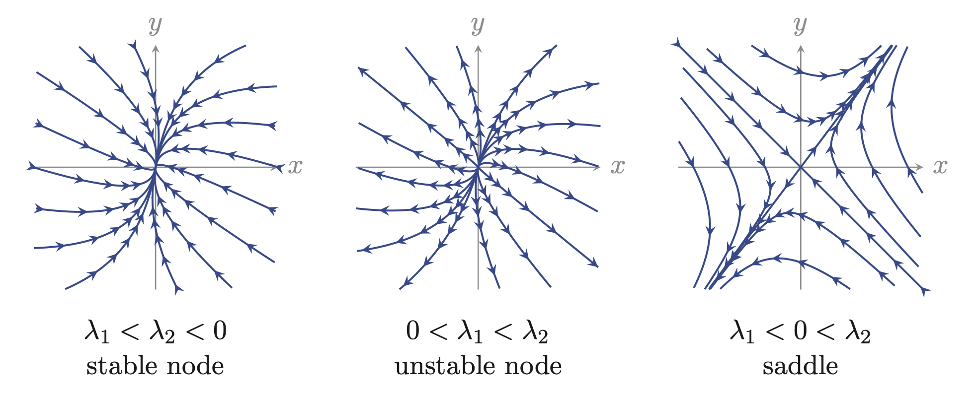
If \(\beta^2 = 4\gamma\) the two eigenvalues, \(\lambda_1\) and \(\lambda_2\), are equal to each other. When \(\beta^2 > 4\gamma\) the eigenvalues are not equal to each other and they are both real valued. Graphical solution to the equation can be illustrated with flow maps (see below figure). When the eigenvalues are both negative (left) the flow will be towards the origin, which represents a stable node. From the solution equation we can see that the flow towards the stable node follows an exponential decay (\(e^{\lambda t}\)). Actually there are two exponential decays: one for each eigenvector. If both eigenvalues are positive the opposite will happen: exponential increase in both directions (middle figure). The last case is where one is positive and one is negative: trajectories will explode in one direction and decay in the other. A physical analogy is a saddle where there is an upward curvature in one directions (which works as stabilizing) and a downward curvature which has an unstabilizing effect in the other direction.

When \(\beta^2 < 4\gamma\) there is not real valued solution to the \sqrt{\beta^2 -4\gamma} part of the eigenvalue polynomium. The means the eigenvalues will now become complex numbers rather than real valued. But what are complex numbers?

3.4. Complex numbers: a short introduction

Complex numbers are a mathematical abstraction with the initial purpose to warrant a solution to equations like the quadratic equation, where there are square roots that can make give problems when you only use real numbers.

Definition: A complex number is typically expressed in the form:

\[ z=a+bi \]

where \(a\) and \(b\) are real numbers. \(i\) is the imaginary unit, defined by the property

\[ i^2=−1 \]

Where real numbers can be represented as a line, complex numbers can be represented graphically on a complex plane, where the horizontal axis represents the real part and the vertical axis represents the imaginary part. Since \(z\) is a point in the complex plane, it can also be represented as a point on a circle:

\[ z=re^{i\theta} \]

Where \(r\) is the radius and \(\theta\) is the angle. Hence, the complex number can both be represented by the numbers, \(r\) and \(\theta\), in a polar representation, or by \(a\) and \(b\) in normal coordinates. Regardless, a complex number is represented by two two real numbers. A last important point: There is a simple relationship between complex numbers and the trigonometric functions sine and consine. That is called Euler’s formula (not to confuse with Euler’s method):

\[ e^{i\theta} = cos(\theta) + isin(\theta) \]

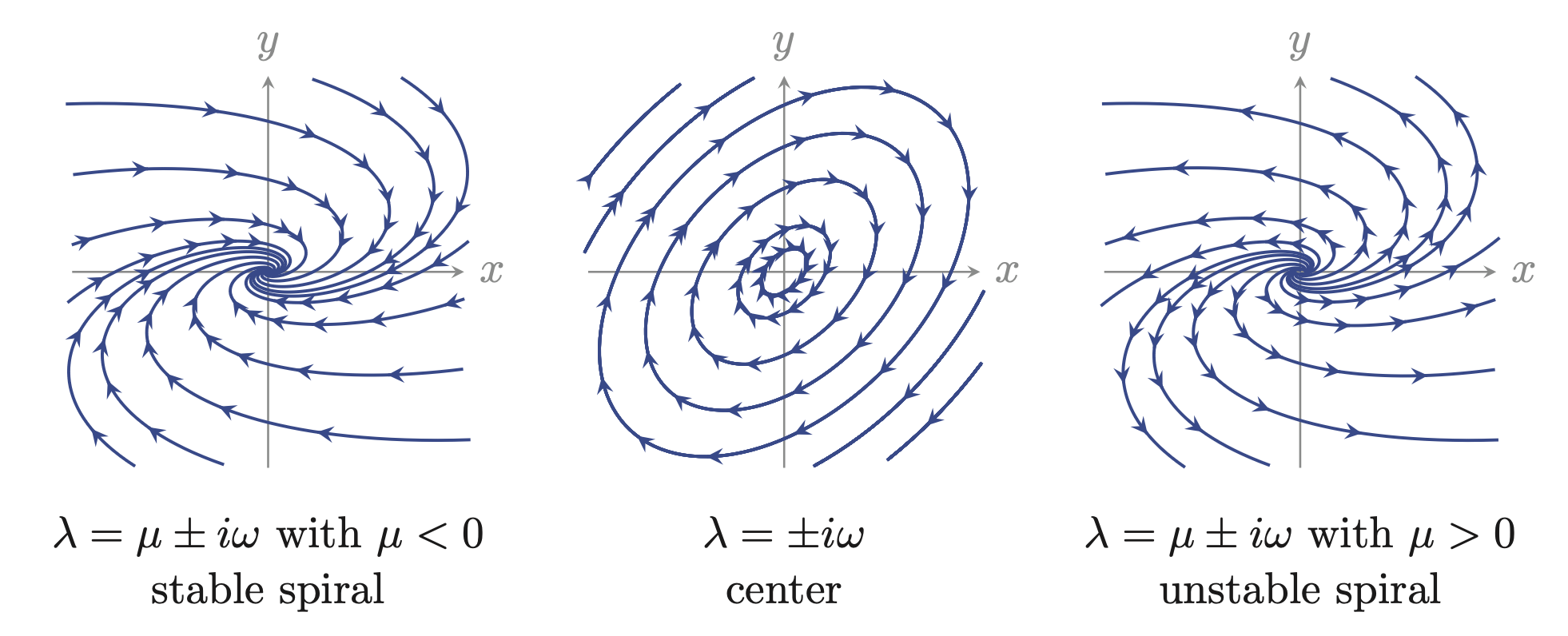
This is where the link to oscillations come in. If the eigenvalues have complex values, then the time dependence of the solution to (1) will have trigonometric functions where the argument is dependent on time. That is oscillations. That bring us back to the when \(\beta^2 < 4\gamma\) . Here, there is not real valued solution to the \(\sqrt{\beta^2 -4\gamma}\) and therefore the eigenvalues are complex numbers, i.e. the \(e^{\lambda t}\) gives a trigonometric contribution. The cases are as shown in the figure below. If \(\mu < 0\) (which is the real part of the eigenvalue) then the solution is rotating and stable, i.e. spiralling inwards (left). If \(\mu =0\) the eigenvalues are purely imaginary, hence there is no exponential decay or explosion. Therefore we get a clean rotation in the state space (middle). When \(\mu > 0\) we get both rotation and exponential increase in amplitude, hence and unstable spiral (right).

3.5. Exercise

Plot first cosine as a function of time. Then plot sine as a function of time. Now plot the same sine versus the same cosine as a function of time.

# Put your code here:

3.6. General solution

The general solution to (1) is actually a sum of the eigenvectors multiplied by the exponential function of the corresponding eigenvalues and time: $\( \vec{x}(t)= c_1\vec{v_1}e^{\lambda_1 t} + c_2\vec{v_2}e^{\lambda_2 t} \)$

where the \(\vec{v_1}\), \(\lambda_1\) and \(\vec{v_2}\), \(\lambda_2\) are the eigenvector and eigenvalue pairs. \(c_1\) and \(c_2\) are real arbitrary constants. In expanded form this can be equivalently written:

\[\begin{split} \begin{bmatrix} x(t) \\ y(t) \\ \end{bmatrix} = c_1 \begin{bmatrix} v_x1 \\ v_y1 \\ \end{bmatrix} e^{\lambda_1 t}+ c_2 \begin{bmatrix} v_x2 \\ v_y2 \\ \end{bmatrix} e^{\lambda_2 t} \end{split}\]

We may note that this can be generalized to higher dimensional systems, where the sum will include more eigenvectors and eigenvalues.

3.7. What does \(Av=\lambda v\) does have to do with \(\dot X = AX\)?

Above we postulate that the eigenvector-eigenvalue equation (\(Av=\lambda v\)) provide the solution for our dynamical system \(\dot X = AX\), and the solution is given as \(ve^{\lambda t}\). This can be understood through the following. We propose \(x(t)=ve^{\lambda t}\) is a solution to \(\dot x = Ax\) if it satisfies the eigenvalue equation \(Av=\lambda v\). Let us see this by inserting the solution in the equation:
$\( \dot x = Ax \)$

\[ \frac{d}{dt}[ ve^{\lambda t}] = A [ve^{\lambda t}] \]

\[ v\frac{d}{dt}[ e^{\lambda t}] = Ave^{\lambda t} \]

\[ v\lambda e^{\lambda t} = Ave^{\lambda t} \]

\[\begin{split} v\lambda = Av \\ Av = \lambda v \end{split}\]

We conclude that \(\dot x = Ax\) has solution \(x(t)= ve^{\lambda t}\) for any vector \(v\) and scalar \(\lambda\) that satisfy the eigenvector-eigenvalue problem \(Av = \lambda v\). The trivial solution \(v=0\) corresponds to the steady state at the origin (x(t)=0).