2. Predator–prey dynamics: Simulation#
Section Credit: Sri Vallabha and Frank Hoppensteadt (2006) Predator-prey model. Scholarpedia, 1(10):1563 under CC BY 3.0 with changes.
In the previous section we have modelled the activity of a single neuron using a single differential equation. What if we want to model the activity of systems with several interacting elements —like a population of neurons? In this case we will need to introduce at least one differential equation per system component. That is, if we have a population of 10 neurons connected to each other —coupled—, we will need at least 10 differential equations to model the whole network activity: we say then that we have a system of coupled differential equations. In the chapter Simulation of neural population, we will do precisely so; but first, let us have a short break from neurons and look at another coupled system
Predator-prey models are a popular model to describe how species intreractions in ecosystems. Species compete, evolve and disperse simply for the purpose of seeking resources to sustain their struggle for their very existence. Depending on their specific settings of applications, they can take the forms of resource-consumer, plant-herbivore, parasite-host, tumor cells (virus)-immune system, susceptible-infectious interactions, etc. They deal with the general loss-win interactions and hence may have applications outside of ecosystems. When seemingly competitive interactions are carefully examined, they are often in fact some forms of predator-prey interaction in disguise.
The Lotka–Volterra equations, also known as the predator–prey equations, are a pair of first-order, non-linear, autonomous* differential equations. They are frequently used to describe the dynamics of biological systems in which two species interact, one as a predator and the other as prey. You can read more about this from Wikipedia http://en.wikipedia.org/wiki/Lotka-Volterra_equation.
Autonomous system or autonomous differential equation is a system of ordinary differential equations which does not explicitly depend on the independent variable, typically dynamical systems are autonomous if the state of the system does not explicitly depend on the time \(t\).
Their populations change with time according to the following pair of equations:
where:
\(x\) is the number of prey (say rabbits),
\(y\) is the number of predators (say foxes).
\(dx/dt, dy/dt\) gives the rate of change of their respective populations over time \(t\).
\(\alpha, \beta, \gamma, \delta \) are the parameters describing the interaction between the two species:
\(\alpha\) is the reproduction rate of species x (the prey) in the absence of interaction with species y (the predators), ie. assuming it’s not predated and has infinite food supply available.
\(\beta\) is the eating rate of predator per prey (equals to the death rate of prey per predator)
\(\gamma\) is the death rate of species y (the predators) in the absence of interaction with species x, eg. if no preys are available.
\(\delta\) is the reproduction rate of predator per prey.
The above equations can be written in a slightly different form to interpret the physical meaning of the four parameters used.
1.Equation for prey
The prey are supposed to have unlimited supply of food and \(\alpha x\) represents the rate of population growth of prey. Rate of decrease of population of prey is assumed to be proportional to the rate at which predator and prey meet and is given by \( \beta y x\)
2.Equation for predator
For the predators, \(\delta x y \) gives the rate of growth of predator population. Note that this is similar to the rate of decrease of population of prey. The second term \(\gamma y \) gives the rate of population decrease for predators due to natural death or emigration.
To solve this system of two differential equations using python, we first need to type the equations as functions as well as it parameters. The function simply needs to return the right hand side of the equations
import numpy as np

# Define the function that represents the Lotka-Volterra equations
def predatorprey(xy, t, alpha, beta, delta, gamma):
    x, y = xy
    dxdt = x * (alpha - beta * y)
    dydt = - y * (gamma - delta * x)
    return np.array([dxdt, dydt])
Now we will use python library Scipy to numerically solve the system. Speciafically we will use the function scipy.integrate.odeint().
# We import scipy ordinary differential equations solver
from scipy.integrate import odeint

#Defined the model parameters
alpha = 1.
beta = 1.2
gamma = 4.
delta = 1.

# Initial population size of each species
x0 = 10.
y0 = 2.
X0 = [x0, y0]

# Simulation timesteps
T  = 30.0                             # final time (the units will depend on what units we have chosen for the model constants)
N = 10000                             # number of time-steps for the simulation
t = np.linspace(0.,T, N)

# Call differential equation solver and stores result in variable res
solution = odeint(predatorprey, X0, t, args = (alpha, beta, delta, gamma))

# Unpack the solution values into two variables
x_solution, y_solution = solution.T
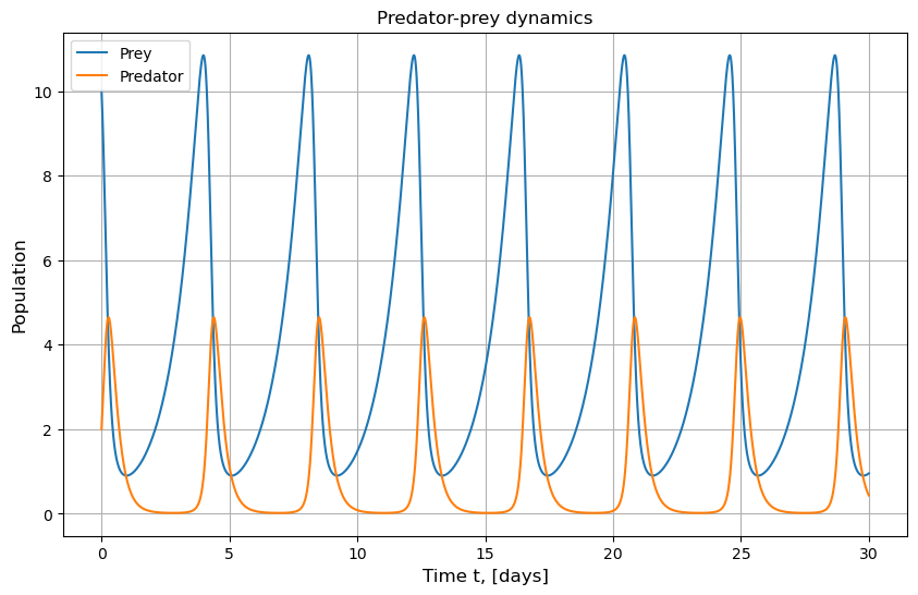
We will now plot the variation of population for each species with time:
from matplotlib import pyplot as plt

plt.figure(figsize=(10, 6))
plt.grid()
plt.title("Predator-prey dynamics")
plt.plot(t, x_solution, label = 'Prey')
plt.plot(t, y_solution, label = "Predator")
plt.xlabel('Time t, [days]', fontsize=12)
plt.ylabel('Population', fontsize=12)
plt.legend()
plt.show()
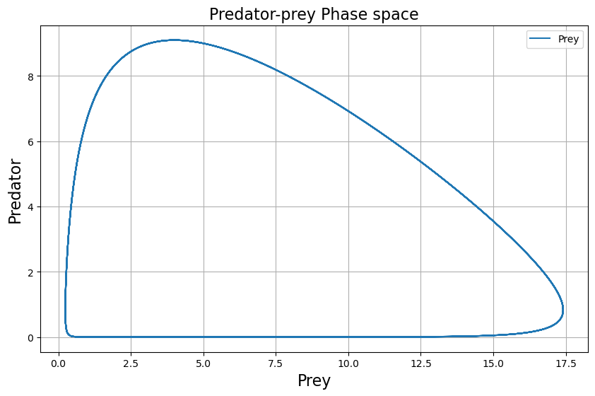
A better understanding of the system behaviour can be obtained by a phase plot of the population of predators vs. the population of prey. It will tell us if the system sustains or collapses over time. For the choice of parameters \( \alpha, \beta, \gamma \) and \( \delta \) made above, we see that the maximum population of each species keeps increasing each cycle. You can read more about that in the Wikipedia link mentioned above.
2.1. Exercises#
Play with parameters to get a sense of the bahaviour of the system and diccuss with your group the system behaviours that you observe. Try to interpret the physical meaning of the changes to the model parameters.
#@title  { run: "auto", vertical-output: true }
alpha = 1.0 #@param {type:"slider", min:0.1, max:4, step:0.1}
beta  = 1.2 #@param {type:"slider", min:0.1, max:4, step:0.1}
gamma = 4.0 #@param {type:"slider", min:0.1, max:8, step:0.1}
delta = 1.0 #@param {type:"slider", min:0.1, max:4, step:0.1}

# Initial population size of each species
preys = 5 #@param {type:"slider", min:2, max:10, step:1}
predactors = 9 #@param {type:"slider", min:2, max:10, step:1}

X0 = [preys, predactors]

# Simulation timesteps
T  = 30.0                             # final time, units depend the constant's units chosen
N = 10000                             # number of time-steps for the simulation
t = np.linspace(0.,T, N)

# Call differential equation solver and stores result in variable res
solution = odeint(predatorprey, X0, t, args = (alpha, beta, delta, gamma))

# Unpack the solution values into two variables
x_solution, y_solution = solution.T

# Plot results
plt.figure(figsize=(14, 8))
plt.grid()
plt.title("Predator-prey solved with scipy odeint", fontsize=16)
plt.plot(t, x_solution, label = 'Prey')
plt.plot(t, y_solution, label = "Predator")
plt.xlabel('Time', fontsize=16)
plt.ylabel('Populations size', fontsize=16)
plt.legend(fontsize=18)
plt.show()
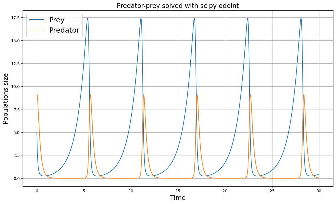
Can you find a set of parameters for which the preyed population become extinct?
2.1.1. Phase space analysis#
If instead of interesting ourselves into how the population evolve overtime, we look at a population value as a function of the other, we call this phase analysis of the system. We can easily plot phase space by plotting the results previously obtained:
plt.figure(figsize=(10, 6))
plt.grid()
plt.title("Predator-prey Phase space", fontsize=16)
plt.plot(x_solution, y_solution, label = 'Prey')
plt.xlabel('Prey', fontsize=16)
plt.ylabel('Predator', fontsize=16)
plt.legend()
plt.show()
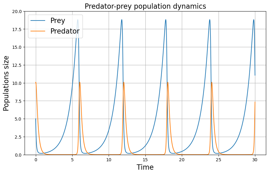
We can also look at both the time evolution and phase representation at the same time. Is the shape of the phase space preserved for different model values?
#@title  { run: "auto", vertical-output: true }
alpha = 1 #@param {type:"slider", min:0.1, max:4, step:0.1}
beta  = 1.2 #@param {type:"slider", min:0.1, max:4, step:0.1}
gamma = 4.0 #@param {type:"slider", min:0.1, max:8, step:0.1}
delta = 1.0 #@param {type:"slider", min:0.1, max:4, step:0.1}

# Initial population size of each species
preys = 5 #@param {type:"slider", min:5, max:20, step:1}
predactors = 10 #@param {type:"slider", min:5, max:20, step:1}

X0 = [preys, predactors]

# Simulation timesteps
T  = 30.0                             # final time, units depend the constant's units chosen
N = 10000                             # number of time-steps for the simulation
t = np.linspace(0.,T, N)

# Call differential equation solver and stores result in variable res
solution = odeint(predatorprey, X0, t, args = (alpha, beta, delta, gamma))

# Unpack the solution values into two variables
x_solution, y_solution = solution.T

# Plot results
plt.figure(figsize=(10, 6))
plt.grid()
plt.title("Predator-prey population dynamics", fontsize=16)
plt.plot(t, x_solution, label = 'Prey')
plt.plot(t, y_solution, label = "Predator")
plt.xlabel('Time', fontsize=16)
plt.ylabel('Populations size', fontsize=16)
plt.ylim(0,20)
plt.legend(fontsize=16)

plt.figure(figsize=(10, 6))
plt.grid()
plt.title("Predator-prey Phase space", fontsize=16)
plt.plot(x_solution, y_solution)
plt.xlabel('Prey', fontsize=16)
plt.ylabel('Predator', fontsize=16)
plt.ylim(0,20)
plt.show()
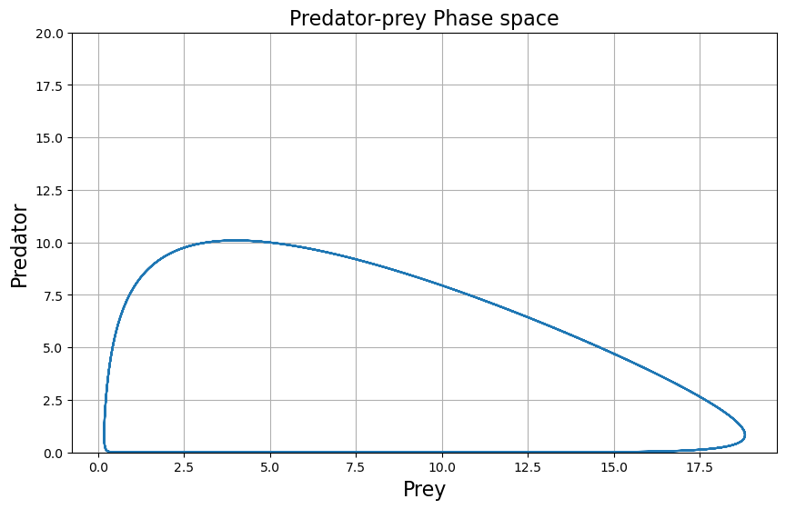
Phase spaces are a powerful tool that allow us to understand the relations between the variables of a dynamical system. Be it relation between predators and preys, between two neurotransmitters or any other dynamical variables.